3.1 Probability Distribution Function

A probability distribution is a mathematical function that describes the probability of different possible outcomes for an experiment. Probability distributions are often depicted using graphs or probability tables.

Probability Distribution Function can be categorized into

• Probability Density Function(PDF)
• Probablity Mass Function(PMF)
• Cumulative Distribution Function(CDF)

3.1.1 Probability Density Function(PDF)

• It describes the probability distribution of a continuous random variable
• Eg:
  • Height of Student

3.1.2 Probablity Mass Function(PMF)

• It describes the probability distribution of a discrete random variable.
• Eg
  • Rolling a dice

3.1.3 Cumulative Distribution Function(CDF)

• It is another method to describe the distribution of a random variable (either continuous or discrete).
• It gives cumulative sum of all the values wrt area under the curve

3.2 Types of Probability Distribution

3.2.1 Bernoulli Distribution

In probability theory and statistics, the Bernoulli distribution, named after Swiss mathematician Jacob Bernoulli, is the discrete probability distribution of a random variable which takes the value 1 with probability p and the value 0 with probability q = 1-p

The probability of occurrence is p and the probability of the event not occurring is 1-p i.e., the event has only two possible outcomes (these can be viewed as Success or Failure, Yes or No and Heads or Tails).

$$P(x=k) = p^k(1-p)^{1-k}$$

$$P(x=1) = p^1(1-p)^1-1 = p$$ $$P(x=0) = p^0(1-p)^1-0 = 1-p = q$$

• Outcome are binary - 0 or 1
• Its Probablity Mass Function(PMF)
• Eg:
  • Tossing a Fair Coin

Mean, Median, Std, Var

Mean

E = Expected value $$E(k) = \sum_{i=1}^{k} k.p(k) $$

E(k) = p

Median = 0, [0,1], 1 for p<1/2, p=1/2, p>1/2

Variance = p(1-p) = pq

Std = sq-root of (pq)

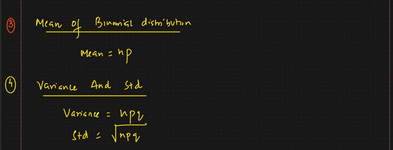
3.2.3 Binomial Distribution

In probablity theory and statistics, the binomial distribution with parameters n and p is a discrete probability of the number of successes in a sequence of n independent experimants, each asking a yes-no question and each with its own boolean-value outcome: success(with probablity p) or failure(with probablity q=1-p).

• Its Probablity Mass Function(PMF)
• Eg:
  • Tossing a coin 10 times

Binomial Distribution related with Bernoulli Distribution.

The binomial distribution is closely related to the Bernoulli distribution.

• A single success/failure experimant is also called a Bernouli trail or Bernoulli experiment.
• And a sequence of outcomes is called a Bernoulli process.

If each Bernoulli trial is independent, then the number of successes in Bernoulli trails has a binomial Distribution. On the other hand, the Bernoulli distribution is the Binomial distribution with n=1.

3.2.3 Poisson Distribution

It describes the number of events occuring in a fixed time interval

• Discrete Distribution
• Its Probablity Mass Function(PMF)
• Eg:
  • No of people visiting hospital every hours
  • No of people visiting bank every hours

$$P(x) = \frac{e^{-\lambda} \lambda^x}{x!}$$

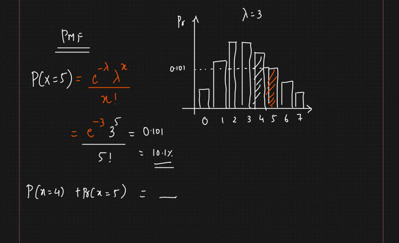
$$ Mean = E(x) = \mu = \lambda * t $$ $$Variance = E(x) = \mu = \lambda * t $$

• Lambda - Expected no of events to occur at every time interval
• t = Time interval
• Mean and Variance is same for Poisson Distribution

3.2.4 Normal/Gaussian Distribution

When the data tends to be around a central value with no bias left or right, and it gets close to a Normal Distribution

• The blue curve is a Normal Distribution.
• The yellow histogram shows some data that follows it closely, but not perfectly (which is usual).
• It is often called a Bell Curve because it looks like a bell.
• Eg:
  • Weight, Height, IRIS dataset

The Normal Distribution has:

• mean = median = mode
• symmetry about the center
• 50% of values less than the mean and 50% greater than the mean
• Its as Symmetric distribution and is Probability Density Function(PDF)

Empirical Rule

• AKA 68–95–99.7 rule or 3 Sigma rule

3.2.5 Uniform Distribution

A uniform distribution is a distribution that has constant probability due to equally likely occurring events. It is also known as rectangular distribution (continuous uniform distribution). It has two parameters a and b: a = minimum and b = maximum.

• There are two types of uniform distribution:
  • Continious Uniform Distribution (pdf)
  • Discrete Uniform Distribution (pmf)

Continuous Uniform Distribution

A continuous uniform probability distribution is a distribution that has an infinite number of values defined in a specified range. It has a rectangular-shaped graph so-called rectangular distribution. It works on the values which are continuous in nature. Example: Random number generator

Probability density function(pdf) - for a ≤ x ≤ b $$P(x) = \frac{1}{(b-a)}$$

Cumulative Distribution function (cdf) - for a ≤ x ≤ b $$ P(x)= \frac{(x-a)}{(b-a)} $$

Mean and Variance $$ Mean(\mu) = \frac{a+b}{2}$$ $$ Variance(\sigma^2) = \frac{(b-a)^2}{12}$$

Discrete Uniform Distribution

A discrete uniform probability distribution is a distribution that has a finite number of values defined in a specified range. Its graph contains various vertical lines for each finite value. It works on values that are discrete in nature. Example: A dice is rolled.

Probability mass function(pmf) - for b >= a $$ pmf = \frac{1}{n}$$ $$Mean = Median = \frac{a+b}{2}$$

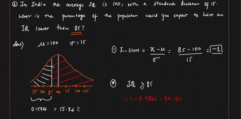
3.2.6 Standard Normal Distribution

The standard normal distribution, also called the z-distribution, is a special normal distribution where the mean is 0 and the standard deviation is 1.

Any normal distribution can be standardized by converting its values into z scores. Z scores tell you how many standard deviations from the mean each value lies.

Normal distribution vs the standard normal distribution

All normal distributions, like the standard normal distribution, are unimodal and symmetrically distributed with a bell-shaped curve.

• Normal distribution can take on any value as its mean and standard deviation.
• In the standard normal distribution, the mean and standard deviation are always fixed.

Every normal distribution is a version of the standard normal distribution that’s been stretched or squeezed and moved horizontally right or left.

The mean determines where the curve is centered. Increasing the mean moves the curve right, while decreasing it moves the curve left.

The standard deviation stretches or squeezes the curve. A small standard deviation results in a narrow curve, while a large standard deviation leads to a wide curve.

Z scores

A z score is a standard score that tells you how many standard deviations away from the mean an individual value (x) lies:

• A positive z score means that your x value is greater than the mean.
• A negative z score means that your x value is less than the mean.
• A z score of zero means that your x value is equal to the mean.

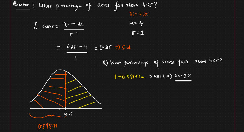
$$ Zscore(z) = \frac{x-\mu}{\sigma}$$

Why standard normal distribution

• All the features in a dataset can be of different units like years(Age), KG(Weight), Cms(Height) …
• For the models/algorithims to work properly all the features are Standardized

Eg: Age, Weight, Height are Standardized as below: $$\frac{x_i-\mu_{Age}}{\sigma}, \frac{x_i-\mu_{Weight}}{\sigma}, \frac{x_i-\mu_{Height}}{\sigma}$$

Z Table

• Z Table PDF
  Previous Next     Page: /

Question

1. What percentage of socres fall above 4.35?

2. In India the avg IQ is 100, with as std of 15. What is the percentage of the population would you expect to have

• an IQ < 85
• an IQ >= 85

Reference

• https://www.statisticshowto.com/probability-and-statistics/statistics-definitions/uniform-distribution/