1.1 Statistics

• Statistics is the science of collecting, organizing and analyzing the data.
• Used for decision making process
• Data - facts or pieces of information

1.2 Types of Statistics

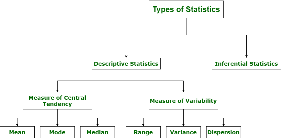
• Descriptive stats
  • It consists of organizing and summarizing the data.
• Inferential stats
  • It consists of using data you have measured to form conclusion, make predictions.
  • By using sample-data make conclusion on population-data

1.2.1 Descriptive stats

• Example
  • Average height of the student in a class (Mean)
  • Most common height in the class(Mode)

Types

• Measure of Central Tendency
  • Mean, Median, Mode
• Measure of Variability
  • Range, Variance, Dispersion, Std
• Charts - Data distribution
  • Histogram, Bar charts

1.2.2 Inferential stats

• Technique used - to form conclusion
  • Z-test
  • T-test
  • Hypothesis testing, P value
• Example
  • Are the avg height of student in the class are similar to what you expect in the entire college
    • class - Sample data, entire college - Population data u

Population vs Sample Data

A population is the entire group that you want to draw conclusions about.

A sample is the specific group that you will collect data from. The size of the sample is always less than the total size of the population.

Why Sample data

Working with sample data is helpful when

• the population is too large or infinite in size
• Size is unknown or not measurable

This is the preferred method of collecting data when the data you need is too hard to gather. It’s a way to get information about the population without actually needing to access every person or item in that population.

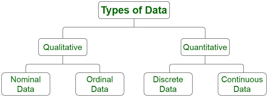
1.3 Types of Data

* Quantitative Data
    * Discrete Data
    * Continuous Data 
* Qualitative Data
    * Nominal Data
    * Ordinal Data

1.3.1 Quantitative/ Numerical Data

• Data is depicted in numerical terms.
• Can be shown in numbers and variables like ratio, percentage, and more.
• Example: 100%, 1:3, 123

Discrete Data

• The type of data that has clear spaces between values is discrete data.
• Whole number, Countable
• There are distinct or different values in discrete data.
• Depicted using bar graphs
• Ungrouped frequency distribution of discrete data is performed against a single value.
• Eg: No of bank acount, No of children

Continuous Data

• This information falls into a continuous series.
• Any Value(int, float), Measurable
• Every value within a range is included in continuous data.
• Depicted using histograms
• Grouped distribution of continuous data tabulation frequencies is performed against a value group.
• Eg: Weight, Height, Temperature

1.3.2 Qualitative/ Categorical Data

• Data is depicted in non-numerical terms.
• Could be about the behavioral attributes of a person, or thing.
• Example: loud behavior, fair skin, soft quality, and more.

Nominal Data

• Nominal data attributes can’t either be ordered or measured

# Examples:
Gender (Women, Men)
Eye color (Blue, Green, Brown)
Hair color (Blonde, Brown, Brunette, Red, etc.)
Marital status (Married, Single)
Religion (Muslim, Hindu, Christian)

Ordinal Data

• Ordinal data is the specific type of data that follows a natural order.

Examples:

Feedback is recorded in the form of ratings from 1-10.
Education level: elementary school, high school, college.
Economic status: low, medium, and high.
Letter grades: A, B, C, and etc.

1.4 Level of Measurement

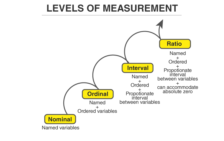
• There are four different scales of measurement.
• The data can be defined as being one of the four scales.

Nominal Scale
Ordinal Scale
Interval Scale
Ratio Scale

1.4.1 Nominal Scale

• It is the 1st level of measurement scale
• It serve as tags or labels to classify or identify the objects.
• Qualitative/Categorical variable
• Order does-not matter
• Example:
  • Gender: M, F
  • Color: Red, Blue, Green

1.4.2 Ordinal Scale

• The ordinal scale is the 2nd level of measurement
• Ordering and ranking matters
• Difference cannot be measured

# Example
Totally agree
Agree
Neutral
Disagree
Totally disagree

# It has ranking and can't calculate difference

1.4.3 Interval Scale

• The interval scale is the 3rd level of measurement scale, which is quantitative.
• Order and Rank matters
• Difference can be measured(excluding ratio)

1.4.4 Ratio Scale

• The ratio scale is the 4th level of measurement scale, which is quantitative
• Order and Rank matters
• Difference and ratio can be measured

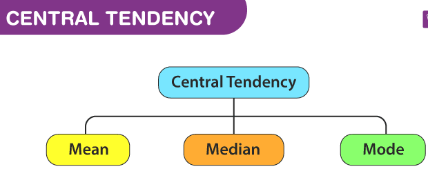
1.5 Measure of Central Tendency

• The central tendency is the descriptive summary of a data set

Mean

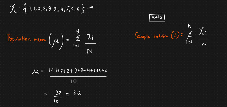
• The mean represents the average value of the dataset.
• It can be calculated as the sum of all the values in the dataset divided by the number of values.

Population mean (Mu) $$ \mu = \sum_{i=1}^{N} \frac{X_i}{N} $$

Sample Mean (s) $$ s = \sum_{i=1}^{n} \frac{X_i}{n} $$

Median

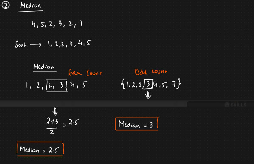
Median is the middle value of the dataset in which the dataset is arranged in the ascending order or in descending order.

When the dataset contains an even number of values, then the median value of the dataset can be found by taking the mean of the middle two values.

Why Median?

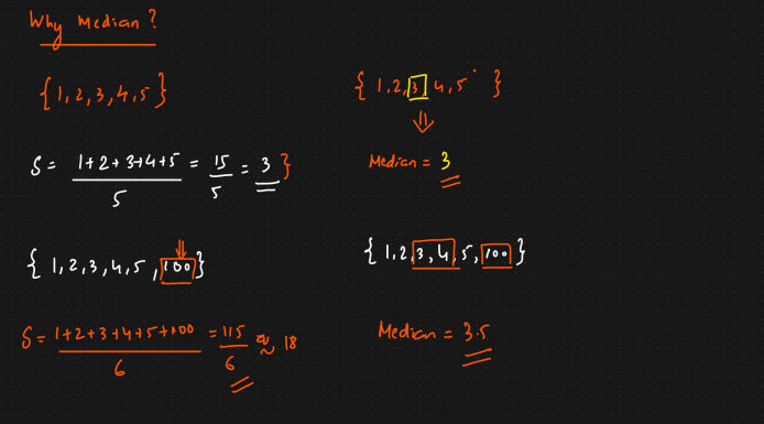
• In case on any outlier in the distribution the
  • mean - huge affect
  • meadian - slight devitaed

Mode

• The mode represents the frequently occurring value in the dataset.
• Sometimes the dataset may contain multiple modes and in some cases no mode at all.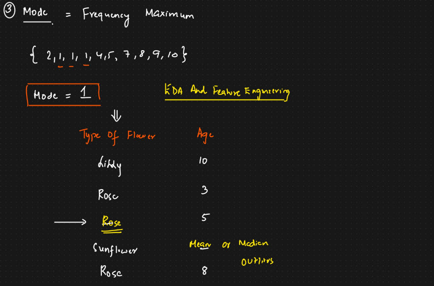

1.6 Measure of Dispersion

• In statistics, the measures of dispersion help to interpret the variability of data i.e. to know how much homogenous or heterogeneous the data is.
• In simple terms, it shows how squeezed or scattered the variable is.

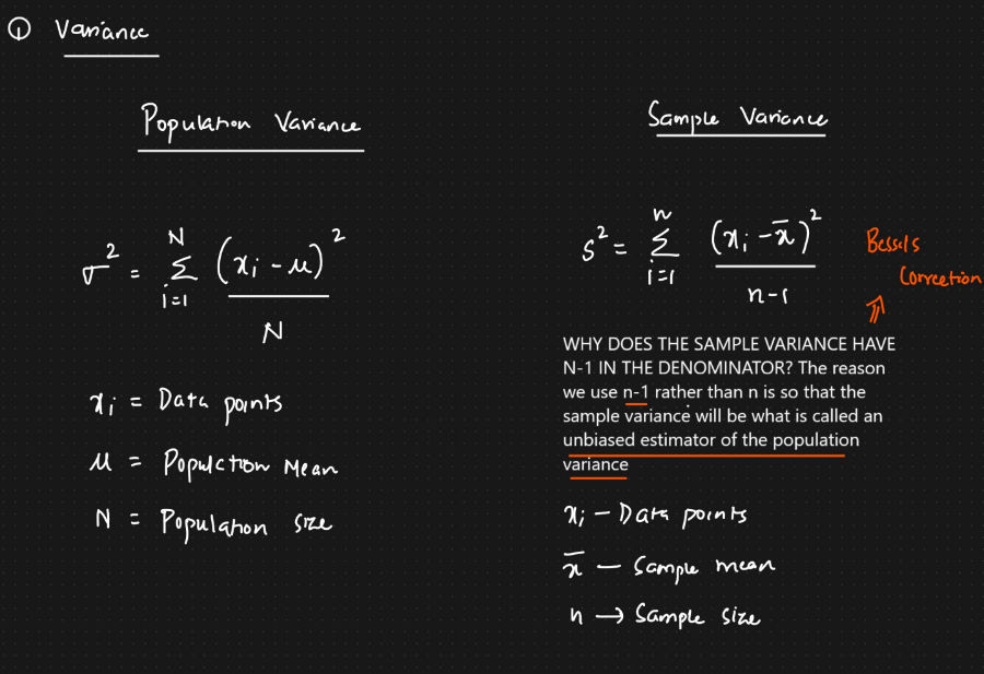
1.6.1 Variance

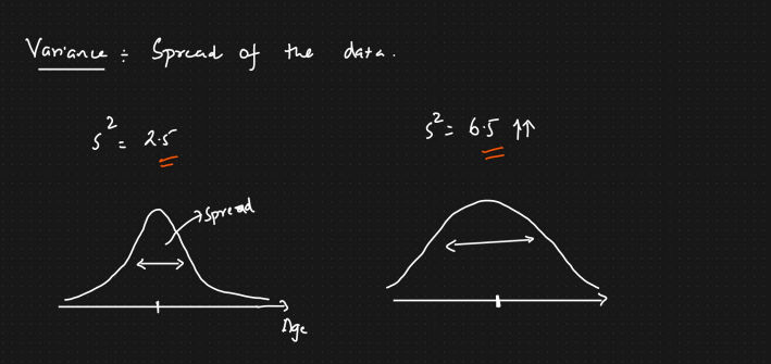
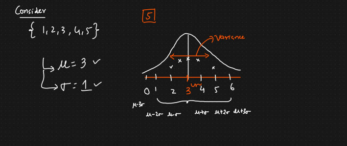
• Spread of data

Population Variance (sigma sq) $$ \sigma^2 = \sum_{i=1}^{N} \frac{(x_i - \mu)^2}{N}$$

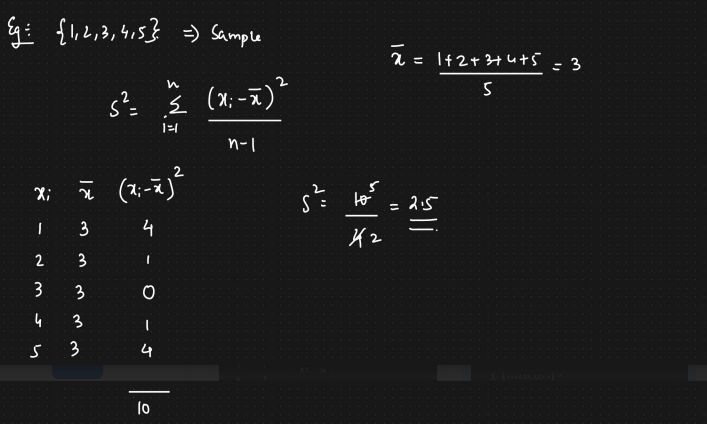
Sample Variance (s sq) $$ s^2 = \sum_{i=1}^{n} \frac{(x_i - \bar{x})^2}{n-1}$$

We use (n-1) rather than n so that the sample variance will be what is called an unbiased estimator of the population variance - Bessels Correction

Example

Variance graph

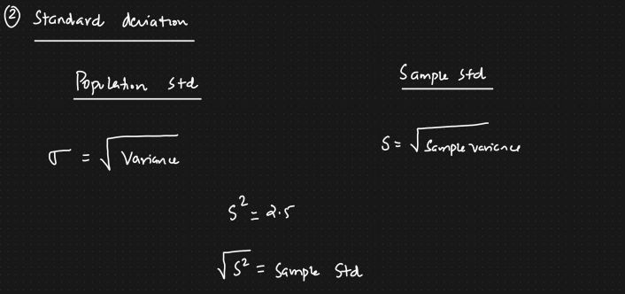
1.6.2 Standard Deviation

Population std (sigma) $$ \sigma = \sqrt{Variance} $$

$$ \sigma = \sqrt{\sum_{i=1}^{N} \frac{(X_i - \mu)^2}{N}} $$

Sample std (s) $$ s = \sqrt{Sample Variance} $$ $$ s = \sum_{i=1}^{n} \frac{(X_i - \bar{X})^2}{n-1}$$

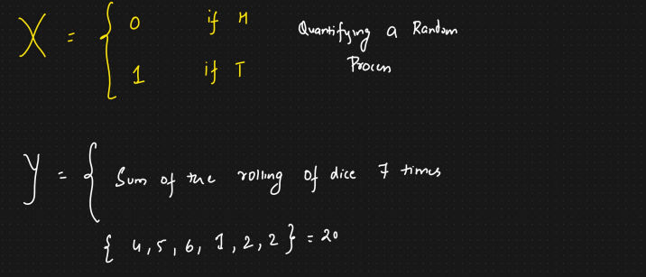
1.6.3 Random Variable

• Random variable is a process of mapping the output of a random process pr expriment to a number
• Eg:
  • Tossing a coin
  • Roling a dice

Below - Value of x, y if fixed i.e x=2 and y=8 $$ x + 5 = 7, x + y = 10 $$

Below - the value of x is not fixed, it depends on the output

Reference

• Types of Statistics
• Types of data in statistics
• Level of Measurement